Model Development

The process of AI model prototype building is a multistep journey that transforms raw data into a functional model. It encompasses several key stages, each playing a crucial role in ensuring the model can learn, generalize, and ultimately perform as required. This section will guide you through the essential steps of engineering, training, and evaluation to create the first model prototype.

While these two stages (Feature Engineering and Model development) are commonly used to describe the model-building process, it’s important to note that there are other ways to segment the workflow. For example, some frameworks emphasize Feature Engineering as distinct stages, while others may break down Model Selection or Hyperparameter Optimization as separate steps. Each approach can vary depending on the complexity of the project and the specific needs of the model being developed.

In this section there is also an optional task where you will be able to build a development pipeline.

This will be the most time consuming section of the workshop, are you ready?

Tools and preparations

In this section we will be using the following tools:

OpenShift AI

OpenShift AI is an integrated platform that simplifies the development and deployment of AI workloads. We will use it to create and manage the Jupyter Notebooks for experimentation and model training. Furthermore, it will enable the creation and orchestration of automated pipelines, ensuring efficient and repeatable workflows.

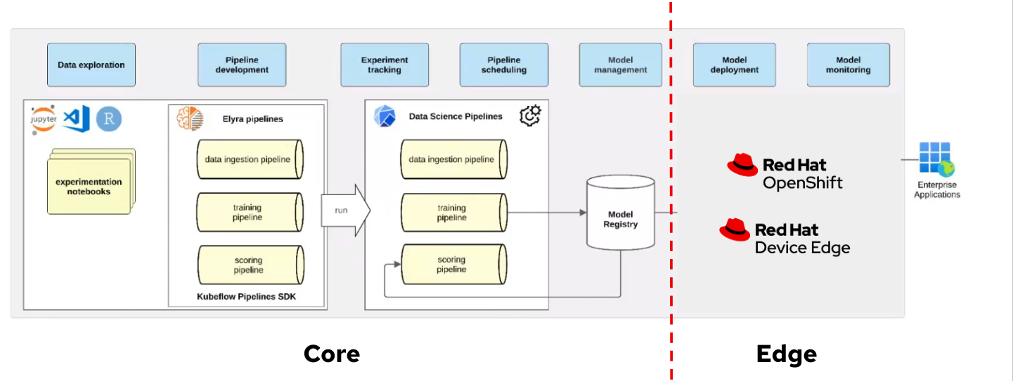
In this workshop we will explore the features of OpenShift AI and their applicability when creating models in OpenShift AI while performing inference on RHEL. OpenShift AI is designed to deploy and serve models directly on OpenShift, leveraging its built-in capabilities for scalability, monitoring, and orchestration. However, it is also possible to leverage OpenShift AI features for workflows where inference is performed on RHEL, or more generic, when inference is performed at the Edge.

When adopting this hybrid approach, you need to bear in mind the following:

Model Compatibility: Ensure the model format is supported by the serving runtime you plan to use on RHEL.
Artifact Retrieval: Model stored in the Object Storage must be exported and transferred to the Edge environment.
Monitoring Integration: Set up a feedback loop to forward inference metrics and logs from RHEL or OpenShift at the Edge to OpenShift AI at the Core/Cloud for analysis is not a built-in feature when performing inference in RHEL.
Security Considerations: Implement secure communication between the Edge and OpenShift AI.

Some features of OpenShift AI will be easier to use when performing inference at the Edge, as they do not require adaptation. For example, using Jupyter Notebooks for model training and export is the same process regardless of the deployment target. However, features such as monitoring or serving will require adjustments to accommodate their use in a RHEL environment, such as setting up Prometheus endpoints or deploying containerized models locally.

In this section Model Building we will be using Data Science Projects and Jupyter Notebooks. OpenShift AI organizes machine learning workflows into projects, providing a collaborative environment for data scientists. Projects integrate Jupyter Notebooks for data preprocessing, model experimentation, and training. It provides a scalable environment with access to GPUs and shared storage.

No real addaptation for these componentes are needed when inference in performed in RHEL, you need to develop and validate models in Jupyter Notebooks and then export the trained model artifacts to the Model Registry or directly to RHEL (explained in Model Serving section).

In the next section Model Serving we will explore additional OpenShift AI features that are useful when preparing your model to be used in RHEL systems (in contrast when you perform the inference in OpenShift)

There are other interesting features such as Distributed Training that are not covered in this workshop.

If you platform has GPUs available, OpenShift and OpenShift AI will be preconfigured to use them.

Source Code Repository (Gitea)

We will use Gitea to store and version-control the Jupyter Notebooks developed for preliminary model training, but any other source code repository such as GitHub could be used.

If you plan to use Gitea you can take a look and check that the "USERNAME-ai" repository is already created:

Navegate to http://gitea.apps.CLUSTER_DOMAIN
Click "Sign In" (top right button) with user "USERNAME" and password "PASSWORD"
You can see on the right the "USERNAME-ai" repository.

Object Storage (OpenShift Data Foundation)

Object storage provides a scalable and accessible solution for persisting large files. Once our model is trained, we will leverage object storage to securely store and manage the model artifacts, ensuring they remain accessible for deployment and further iterations.

In this workshop OpenShift Data Foundation, an Open Source High Performance Object Storage, is deployed in the environment and two object buckets have been created, one to store the AI models (USERNAME-ai-model) and other that will be used by the AI Pipelines USERNAME-ai-pipelines

Feature Engineering

Feature Engineering is the foundation of the model building process, where data and features are prepared and transformed into a form that can be consumed by the model. This stage involves selecting appropriate algorithms and designing architectures.

Selecting appropriate algorithms involves analyzing the problem type, such as classification or regression, and understanding the data’s characteristics to identify the best-fit solution. This process requires balancing performance metrics like accuracy, interpretability, and computational efficiency through experimentation. Designing architectures focuses on defining the structure of the model by choosing the right combination of layers, activation functions, and hyperparameters to capture the complexity of the data.

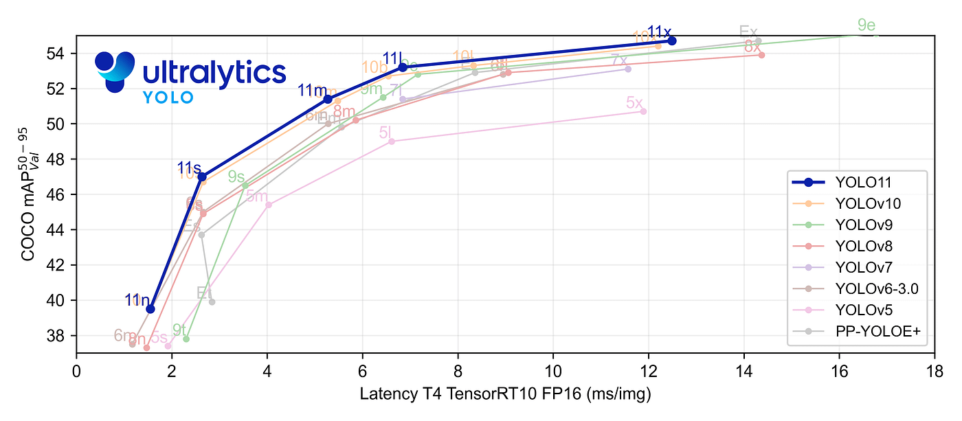
We already explained that our project involves a classification problem, and that the pre-selected algorithm is YOLO on its version 11. YOLOv11 (You Only Look Once, version 11) is the latest evolution in the YOLO family of object detection models, building on its predecessors to achieve faster and more accurate results. This model is designed to meet the growing demands of near real-time object detection applications in fields such as autonomous vehicles, video surveillance, robotics, and more.

During the dataset preparation phase, we incorporated essential feature engineering steps, including balancing the dataset, ensuring high-quality annotations, applying augmentations like flipping, scaling, and mosaic augmentation, and normalizing image sizes. These steps laid a robust foundation for our data.

However, these aspects can also be revisited and refined during feature engineering to further enhance model performance. Additionally, during model development, we can introduce advanced augmentation and preprocessing techniques not included in the data management phase, such as domain-specific augmentations, fine-tuned normalization strategies, or even dynamically generated transformations, tailored to YOLOv11’s capabilities.

This step requires no actions in this workshop, as these aspects were reviewed and addressed during the Data Management phase, just bear in mind that you cound need to revisit them as part of the Model Development cycle to obtain a better performance.

Model Development

At this stage, it is essential to focus on choosing the right hyperparameters during training, such as the learning rate, batch size, input image size, number of epochs, optimizer, etc. These parameters significantly impact the model performance, and fine tuning them is critical for achieving optimal results. Prototyping plays a crucial role in this process, allowing you to experiment with various configurations and refine model architectures iteratively. A common and effective way to perform this experimentation is by using Jupyter Notebooks.

Jupyter Notebooks are an interactive computing environment that combines live code, visualizations, and narrative text in a single document. They are ideal for prototyping machine learning models because they allow you to quickly test, debug, and document your workflows in a user-friendly interface.

To get started, you will create a new, empty Jupyter Notebook using OpenShift AI. In order to do so you have to

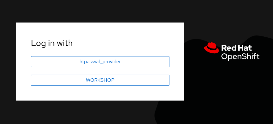
1- Navegate to https://rhods-dashboard-redhat-ods-applications.apps.CLUSTER_DOMAIN

2- Log in using your OpenShift credentials: USERNAME / PASSWORD. It’s a good idea to refresh the page right after the first log in in order to let the left menu load completly with all the additional enabled features.

You need to select the WORKSHOP authenticaticator

3- Open the Data Science Project "USERNAME-ai".

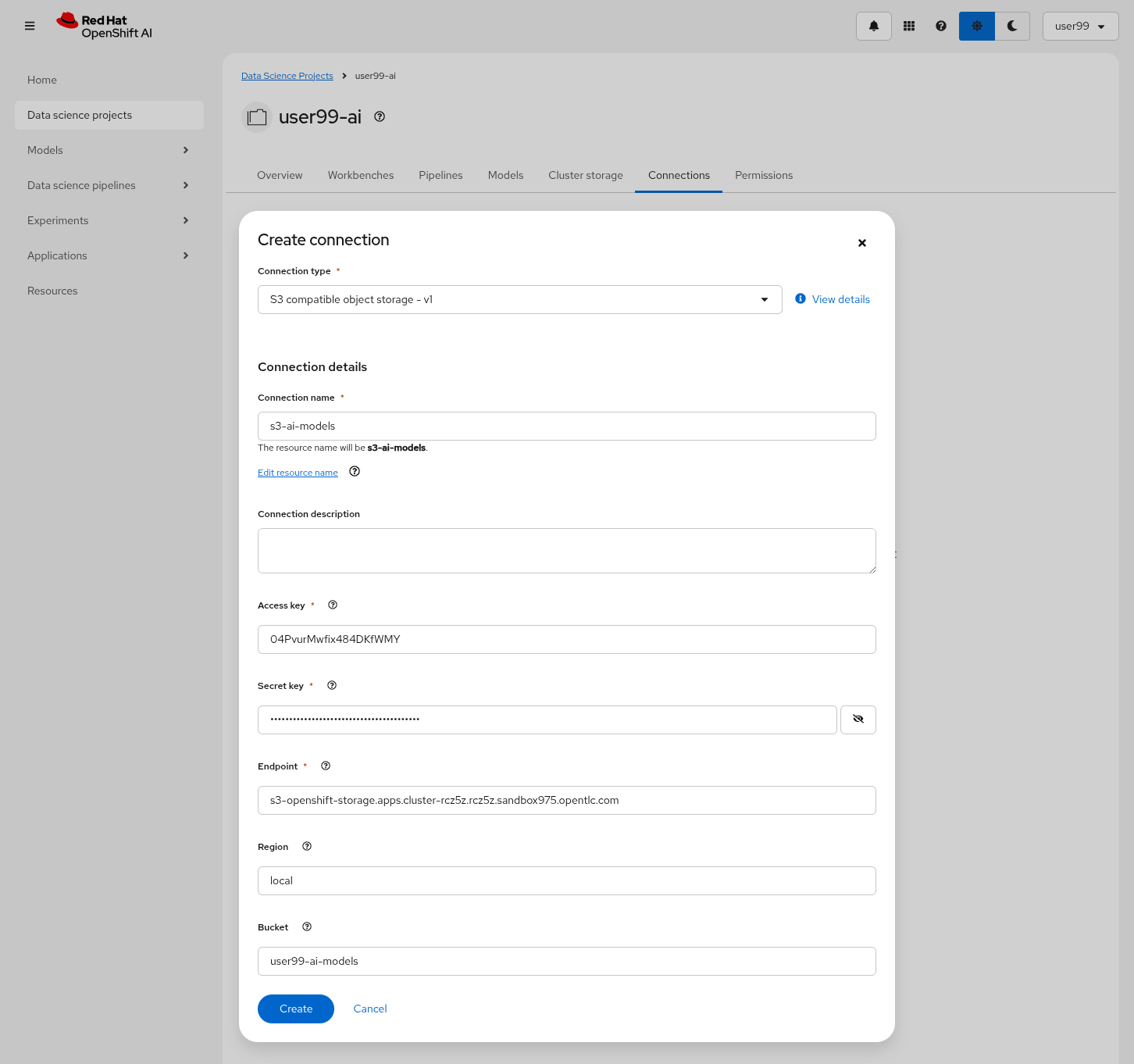
4- Create a new S3 Storage Connection ("Connetions" tab) that will be used by your Jupyter Notebooks to save the model and performance stats. Include:

Name for the S3 connection: We suggest using s3-ai-models
Access key: OBJECT_STORAGE_MODELS_ACCESS_KEY
Secret key: OBJECT_STORAGE_MODELS_SECRET_KEY
Endpoint: s3-openshift-storage.apps.CLUSTER_DOMAIN
Region: You can keep the Region. If it is empty but it’s better to include any string (e.g. local).
Bucket: USERNAME-ai-models

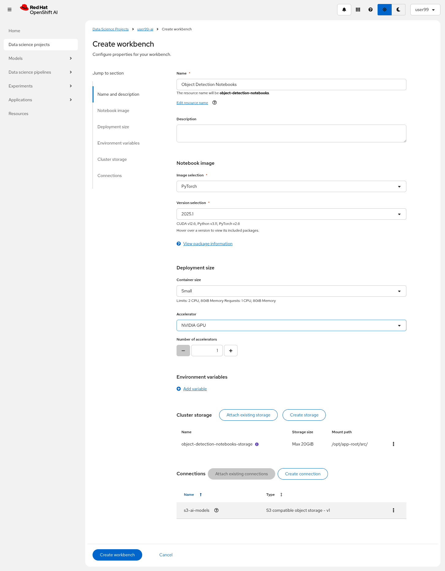
5- Create a new Workbench ("Workbenches" tab) named Object Detection Notebooks. You will need to select:

Base image that will be used to run your Jupyter Notebooks (select PyTorch)
Container Size (Small is enough)
Persistent Volume associated to the container (you can keep the default 20Gi Persistent Volume for your Notebook but you won’t need that much storage)
Object Storage Connection that you already configured.
Additionally, when you have GPUs you will find that during the Workbench creation you also can use accelerators (see an example below with NVIDIA GPUs).

6- Click "Create Workbench". It will take some time to create and start it.

7- Once started, open the Workbench (it could take time to open). You will be asked to allow permissions pior to show the Jupyter environment in your browser.

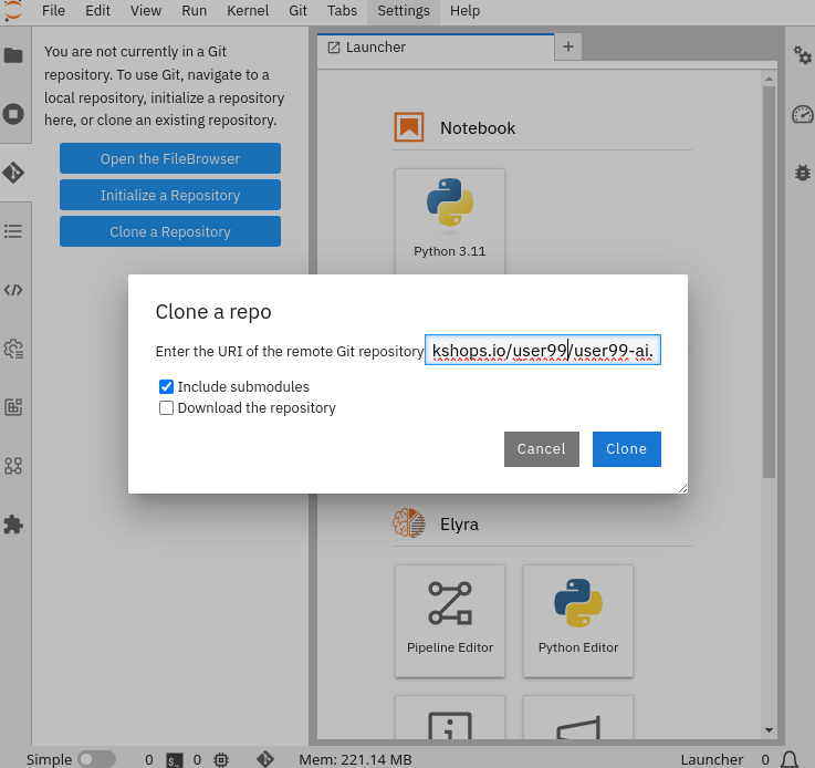
8- Clone the source code repository that you created ("USERNAME-ai") using the left menu (you can find the repository clone URL opening the Gitea repository). Once you click "Clone" a message will appear in the button right. It could take some time to clone the repository.

9- Create a prototype.ipynb file inside the cloned directory ("USERNAME-ai")

It’s time to begin working on the Jupyter Notebook you just created. Below, you will find subsections that explain each necessary code block. To get started, create new code blocks by clicking the + button in the top menu. Configure each block based on the instructions provided below, then run the block by clicking the play button (> icon) to ensure it works as expected. You are encouraged to add additional Markdown cells for further explanations or adjust the provided code to suit your needs. This hands-on approach will help you gain a deeper understanding and tailor the notebook to your specific project.

Let’s start with the first code block, the dependencies.

If you’d prefer to skip the process of configuring each code block or simply want to see the completed version, the full Jupyter Notebook is available for you to review here. This allows you to quickly access the final file without spending time on the setup.

Dependencies

When setting up the Workbench to run your Jupyter Notebook, you were required to select one of the available base container images (e.g., Pytorch). The Jupyter Notebook will execute within this environment, which means all the pre-installed packages and tools in that container image will be readily available.

In our case, however, we will need additional packages, such as the one that allows accessing the dataset directly from Roboflow. These packages may not be included in the selected base image, so it’s essential to install them manually. You can do this by running the following pip install command:

# For Training
!pip install ultralytics roboflow

Once you have identified all the required packages, consider creating a custom base image that includes these dependencies (check the Software included in the supported workbench images). This optimized image will streamline not only the prototyping phase but also regular training workflows performed through Pipelines.

Python Libraries

Import all necessary libraries for training and analysis. Basically you will need:

Libraries for training:

This block will be dependant on your Python code, but probably you will need the following imports:

# Common
import  os

# For Dataset manipulation
import yaml
from roboflow import Roboflow

# For training
import torch
from ultralytics import YOLO

# For Storage
import boto3
from botocore.exceptions import NoCredentialsError, PartialCredentialsError

Roboflow Dataset download

The next step is to download the dataset prepared in the Data Management section. Instead of manually downloading the ZIP file, we will access the dataset directly from Roboflow for a more streamlined process. When you created the "Roboflow Version" of the dataset, you received a unique code to access it. Now, it’s time to put that code to use.

Double check that you’re using the correct API Key, Workspace name, Project name, and Version number to ensure a seamless connection to the dataset.

If you have multiple versions of your dataset, make sure you are using the correct version number under project.version. For example, if you created a new version as part of the "Mock Training" (training the model with a smaller dataset), verify that the version matches the intended dataset.

from roboflow import Roboflow

rf = Roboflow(api_key="xxxxxxxxxxxxxxxxx")  # Replace with your API key
project = rf.workspace("workspace").project("USERNAME-hardhat-detection") # Replace with your workspace and project names

version = project.version(1) # Replace with your version number
dataset = version.download("yolov11")

This code downloads the Dataset, but you’ll need to explicitly specify the paths to each data split (training, validation, and test) in the Dataset metadata. This ensures YOLO can correctly locate and utilize your dataset files.

This is done in the data.yaml file. Open that file so you can see the paths that you need to update by removing the dots and completing the path:

train: ../train/images
val: ../valid/images
test: ../test/images

You can reuse this code block to do it automatically if you don’t want to open and update the file manually:

dataset_yaml_path = f"{dataset.location}/data.yaml"

with open(dataset_yaml_path, "r") as file:
    data_config = yaml.safe_load(file)

data_config["train"] = f"{dataset.location}/train/images"
data_config["val"] = f"{dataset.location}/valid/images"
data_config["test"] = f"{dataset.location}/test/images"

with open(dataset_yaml_path, "w") as file:
    yaml.safe_dump(data_config, file)

Hyperparameter configuration

It’s time to prepare our first model prototype, and for that, you’ll need to configure the hyperparameters for the first iteration of training.

Model hyperparameters are key configuration settings that define how a machine learning model will be trained. These settings are chosen before training begins and significantly affect the model’s performance and efficiency during the training process.

Here are the main hyperparameters you can tune for your YOLO model, along with brief explanations and approximate values to help guide you through the setup:

The list below is a subset of all the parameters that you can configure. You can find all the YOLO training configuration options here, including default values and a short explanation.

Training Settings

Batch size (batch): The batch size is the number of training samples used in one forward and backward pass. A larger batch size leads to more stable gradients and will also reduce sustantially the training time but requires more memory. Value will be dependant on your hardware (mainly memory) that you have available in your CPU/GPU, typical values are 16, 32 or 64. You can try higher values if your GPU allows it. Take into account that if you are running the training on your CPU and configure a batch size that your container instance size cannot manage,then the Workbench will launch an error while training the model and will ask if you want to restart it.

If batch size is a large number you could have not enough memory in your GPU or system to accomodate it, so the training task will fail. You will see a "not enough memory" message in the log.

Epochs (epochs): The Epochs are the number of complete passes through the entire training dataset. More epochs generally improve model performance but also increase training time and risk of overfitting. Typical values: 50, 100 (default), 300. Start with 50 and increase if needed (or just configure 1 epoch if you are running the "Mock Training").
Base YOLO Model (model): The base model architecture, which defines the neural network’s structure. For YOLO, different versions (e.g., YOLOv4, YOLOv5) or sizes (e.g., YOLOv5s, YOLOv5m) can be selected depending on your requirements. In our project we will base our model in YOLOv11 so you will need to configure yolo11m.pt.
Image Size (imgsz): The resolution of the images fed into the model during training. Higher resolutions improve accuracy but increase training time and memory usage. Typical values: 640 (default), 1280. Start with 640 and increase if your system can handle larger images.
Patience (patience): Patience is the number of epochs with no improvement in validation performance before the early stopping mechanism kicks in to stop training. This helps prevent overfitting by stopping training early. Typical value is 10 but try to increase the value if you hit the early stopping, to be sure that you are not preventing the training to make your model improve in later epochs.

Optimization Parameters

Optimized (optimizer): The algorithm used to minimize the loss function during training. Common optimizers include Adam and SGD (Stochastic Gradient Descent) being Adam the default. You never know which one could be better so configure either Adam or SGD and check the results in each case.
Learning rate (lr0 and lrf): The learning rate controls how quickly the model updates weights during trainicng. Adjusting the learning rate can significantly impact model performance and training time. A learning rate that is too high may cause the model to converge too quickly to a suboptimal solution or fail to converge, while a rate that is too low can slow down training and may result in underfitting. You have two values, the first one is lr0, the starting learning rate used at the beginning of the training process and that determines the size of the initial updates made to the model weights during gradient descent. The other value is lrf, the Learning Rate Final Multiplier, that is a multiplier that specifies the final learning rate as a fraction of lr0, the learning rate gradually decays from lr0 to lr0 * lrf over the course of training. Typical values are 0.01 for both parameters. If the model takes too long to converge, consider increasing the learning rate. However, if you observe sudden fluctuations or jumps in performance, it may indicate the need to reduce the learning rate (ie. lr0 = 0.001) to facilitate smoother and more stable convergence.
Momentum (momentum): Momentum is a method used in training models to make learning faster and smoother. Instead of just using the current error to update the model, it also remembers the direction it was going in before and if continues in the same directio the learning rate is increased. This helps the model move more steadily, avoid bouncing around too much, and speed up when progress is slow. Default value is 0.937
Weight Decay (weight_decay): Also known as L2 regularization. Weight Decay is a technique that adds a penalty to the loss to prevent overfitting by discouraging large weights. The idea is to encourage the model to keep the weights small, which can lead to simpler, more general models that perform better on unseen data. The default value is 0.0005.
Warmups (warmup_epochs, warmup_bias_lr, warmup_momentum): Warmups gradually increase the learning rate during the first few epochs to help the model stabilize before it starts learning aggressively. You have three hyperparameters: warmup_epochs, warmup_bias_lr, warmup_momentum. The warmup_epochs (default 0.8) is the number of steps where the learning rate gradually increases, warmup_bias_lr (default 0.1) controls the initial learning rate for bias parameters during warmup, and warmup_momentum (default 3.0) sets the starting momentum value, all helping to stabilize the model’s early training.
Automatic Mixed Precision (amp): Deep Neural Network training has traditionally relied on IEEE single-precision format, however with Automatic Mixed Precision, you can train with half precision while maintaining the network accuracy achieved with single precision. It’s useful for saving memory and speeding up computations but sometimes its usage cause issues with certain GPUs. Defaults to True.

Additional Model Configuration

Name (name): The name of the experiment or model version. It helps to track and differentiate between different training runs.
Dataset path (data): The path to the dataset used for training. This includes both training and validation datasets.
Device used (device): The device used for training. Specify whether you are using a CPU or GPU. If using GPU, make sure it’s set to cuda.

Besides the hyperparameters above, you can also introduce Data Augmentation settings (additional to the Data Augmentation that you could have applied into your Dataset during the Data Management section). Check below the options that you have and the default values.

If you plan to introduce additional Data Augmentation be sure that you set 'augment` to True in order to apply these configurations.

    # Data augmentation settings
    'augment': True,
    'hsv_h': 0.015,  # HSV-Hue augmentation
    'hsv_s': 0.7,    # HSV-Saturation augmentation
    'hsv_v': 0.4,    # HSV-Value augmentation
    'degrees': 10,    # Image rotation (+/- deg)
    'translate': 0.1, # Image translation
    'scale': 0.3,    # Image scale
    'shear': 0.0,    # Image shear
    'perspective': 0.0,  # Image perspective
    'flipud': 0.1,   # Flip up-down
    'fliplr': 0.1,   # Flip left-right
    'mosaic': 1.0,   # Mosaic augmentation
    'mixup': 0.0,    # Mixup augmentation

Now that you’re familiar with the configuration parameters, the goal of this code block is to define and configure a variable (CONFIG) that consolidates all your tuning adjustments (other than defaults).

CONFIG = {
    'var1': 'value1',
    'var2': 'value2',
    ...
    ...
    ...
    'varn': 'valuen',
}

Make your initial guesses for the hyperparameter values for the first model training (next code block). Then, iteratively come back to this code block and adjust and fine-tune these values, retraining the model each time, with the goal of achieving improved performance.

Model Training

Starting the model training with a base model like YOLO is beneficial because it’s pretrained on large datasets, making it faster, more accurate, and less data intensive than training from scratch. Base models provide optimized architectures and learned general features (e.g., edges, shapes) that can be adapted to your specific task thanks to Transfer Learning.

Transfer learning reuses a model trained on one task for another. Early layers retain general features, while later layers are fine tuned for task-specific objects. This approach saves time, requires less data, and leverages pretrained knowledge for better performance.

The first task in this block is to load that base YOLO model. If you remember, you created a variable with the base model name (CONFIG['model']) in the previous block, now it is time to use it:

model = YOLO(CONFIG['model'])

Now it’s time to start the most time consuming task, the model training. You have to use the variables configured in the previous block. In order to save time, you can find below the code block that will do it for you.

By default, the train method of the YOLO library handles both "Training" and "Validation" Data Sets, so you will see results for both in the output.

results_train = model.train(
    name=CONFIG['name'],
    data=CONFIG['data'],
    epochs=CONFIG['epochs'],
    batch=CONFIG['batch'],
    imgsz=CONFIG['imgsz'],
    patience=CONFIG['patience'],
    device=CONFIG['device'],
    verbose=True,

    # Optimizer parameters
    optimizer=CONFIG['optimizer'],
    lr0=CONFIG['lr0'],
    lrf=CONFIG['lrf'],
    momentum=CONFIG['momentum'],
    weight_decay=CONFIG['weight_decay'],
    warmup_epochs=CONFIG['warmup_epochs'],
    warmup_bias_lr=CONFIG['warmup_bias_lr'],
    warmup_momentum=CONFIG['warmup_momentum'],
    amp=CONFIG['amp'],

    # Augmentation parameters
    augment=CONFIG['augment'],
    hsv_h=CONFIG['hsv_h'],
    hsv_s=CONFIG['hsv_s'],
    hsv_v=CONFIG['hsv_v'],
    degrees=CONFIG['degrees'],
    translate=CONFIG['translate'],
    scale=CONFIG['scale'],
    shear=CONFIG['shear'],
    perspective=CONFIG['perspective'],
    flipud=CONFIG['flipud'],
    fliplr=CONFIG['fliplr'],
    mosaic=CONFIG['mosaic'],
    mixup=CONFIG['mixup'],
)

Remember to use the "Mock Training" Dataset if you want to save time while trying this step.

Once the training is done you can see how a new directory has been created under ./run/detect. If you open that directory you will find:

Subdirectory weights with files representing the model with best metrics (best.pt) and the model of the last iteration (last.pt).
Sample images with detections for some inputs of the test and validation sets.
File args with the hyperparameters used during training.
A serie of graphs and schemas along with a file results.csv with the results of the model training and validation.

You can find an example of these files here.

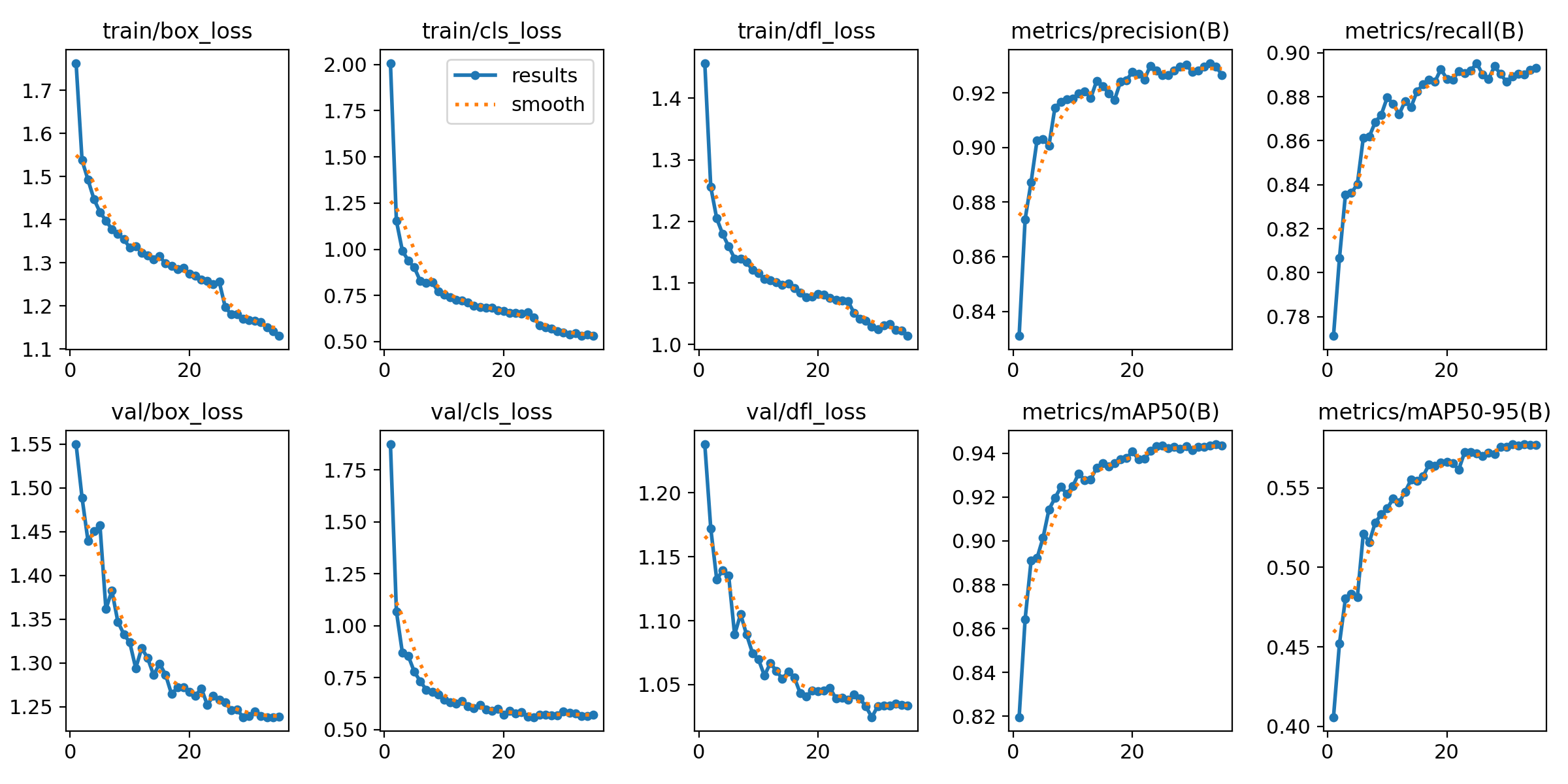
Those graphs are automatically generated by the YOLO method from the results.csv and include:

Confusion Matrix and Confusion Matrix Normalized: A table that shows the true positives, false positives, false negatives, and true negatives for each class. The normalized version represents values as proportions, aiding in comparisons across classes with varying sample sizes.
F1 Curve: A graph plotting the F1 score (harmonic mean of precision and recall) against confidence thresholds, highlighting the balance between precision and recall across different thresholds.
P Curve (Precision Curve): A plot of precision (ratio of true positives to predicted positives) across varying confidence thresholds, indicating the model’s ability to make accurate predictions.
R Curve (Recall Curve): A plot of recall (ratio of true positives to actual positives) across confidence thresholds, showing the model’s ability to identify all instances of a class.
PR Curve (Precision-Recall Curve): A graph that visualizes the trade-off between precision and recall at different thresholds, providing insights into the model’s performance across confidence levels.
Labels Correlogram and Stats: A heatmap illustrating the co-occurrence of labeled objects in the dataset, combined with statistical summaries of label distributions and relationships, helping identify biases or correlations in the training data.
Epoch Steps Summary Results: A summary of key metrics recorded at each training epoch, including others such as:
- Train/Box Loss: The loss related to bounding box regression accuracy.
- Train/Cls Loss: The loss associated with classification errors.
- Train/DFL Loss: Distribution Focal Loss, used for accurate bounding box localization.
- mAP@50: Mean Average Precision at IoU threshold 0.5, measuring detection performance.
- mAP@50-95: Mean Average Precision averaged across IoU thresholds from 0.5 to 0.95, indicating overall model precision and recall.

You will also find in that directory under weights two files (models), one with the best performance obtained (best.pt) and another one created as result of the last epoch iteration (last.pt).

Model Evaluation

Model evaluation using the test split is the process of assessing a trained model’s performance on a subset of data (the test set) that the model has never seen during training or validation. This step provides an unbiased estimate of how well the model will perform on new, unseen data.

results_test = model.val(data=CONFIG['data'], split='test', device=CONFIG['device'], imgsz=CONFIG['imgsz'])

After the evaluation with the Test Data Set you will see how a new directory with the results, similar to what you got with the training, has been created.

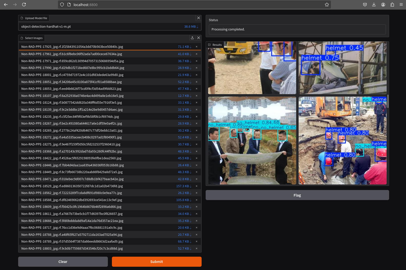
To visually test the performance of your object detection model, you can download the best.pt file (check the directory runs/detects/<model_name>/weights). Then, utilize the following containerized application to perform the test locally: object-detection-batch-model-file.py. This script allows you to run a visual model performance evaluation directly on your local machine.

podman run -p 8800:8800 quay.io/luisarizmendi/object-detection-batch-model-file:latest

The image includes PyTorch dependencies, making it quite large. As a result, the pull process may take some time to complete.

Or if you have an NVIDIA GPU:

podman run --device nvidia.com/gpu=all --security-opt=label=disable --privileged -p 8800:8800 quay.io/luisarizmendi/object-detection-model-test:latest

If you find the following error:

Error: crun: cannot stat /usr/lib64/libEGL_nvidia.so.565.57.01: No such file or directory: OCI runtime attempted to invoke a command that was not found

Be sure that you have ran sudo nvidia-ctk cdi generate --output=/etc/cdi/nvidia.yaml

The application takes some time to start.

It will be ready when you get this log in the terminal:

Creating new Ultralytics Settings v0.0.6 file ✅ View Ultralytics Settings with 'yolo settings' or at '/app/.config/Ultralytics/settings.json' Update Settings with 'yolo settings key=value', i.e. 'yolo settings runs_dir=path/to/dir'. For help see https://docs.ultralytics.com/quickstart/#ultralytics-settings.

Once it’s up you can navigate to http://localhost:8800/ and the select the file with the model and all the images where you want to test it (you can download the Dataset from Roboflow as explained in the Data Management section and use the Test Set)

Drag-and-drop does not work with Chrome, if you use that browser click on the box and select manaully the files, otherwise you will see them as with a size of 0 bytes.

Model Export (optional)

Model export is the process of saving or converting a trained machine learning model into a specific format that can be used for inference or deployment in different environments. This is important because it allows the trained model to be shared, deployed to production, or used in different applications without needing the original training code or environment.

For example, ONNX (Open Neural Network Exchange) is a popular open-source format that is designed for the interchange of deep learning models across different frameworks (ie. OpenVINO), so in this example we are going to convert the Pytorch .py file into the onnx format.

The good news is that the YOLO library provides an export method that makes this possible with just one line:

model.export(format='onnx', imgsz=CONFIG['imgsz'])

Once that’s done, you can review again the weights directory and you will see the new onnx file.

Store the Model

The last code block example that we will see is the one used to store the results (models and metrics) of this prototyping run.

In order to do that you need to create an Object Storage Client and then use it with the files that you can upload. We are using OpenShift Data Foundation as Storage Object:

s3_client = boto3.client(
    "s3",
    endpoint_url=f"https://{AWS_S3_ENDPOINT}",
    aws_access_key_id=AWS_ACCESS_KEY_ID,
    aws_secret_access_key=AWS_SECRET_ACCESS_KEY,
    verify=True
)

But what are those values? Well, when you created the Workbench you configured an "Storage Connection" with details about the Object Storage. These values were injected as Environment variables that now you can use, so before the client setup you will need to import them as follows:

AWS_S3_ENDPOINT = os.getenv("AWS_S3_ENDPOINT", "").replace('https://', '').replace('http://', '')
AWS_ACCESS_KEY_ID = os.getenv("AWS_ACCESS_KEY_ID")
AWS_SECRET_ACCESS_KEY = os.getenv("AWS_SECRET_ACCESS_KEY")
AWS_S3_BUCKET = os.getenv("AWS_S3_BUCKET")

Once you have the Object Storage Client configured, you just need to select the files and upload them using the client.fput_object method:

model_path_train = results_train.save_dir
weights_path = os.path.join(model_path_train, "weights")
model_path_test = results_test.save_dir

# Get file lists
files_train = [os.path.join(model_path_train, f) for f in os.listdir(model_path_train) if os.path.isfile(os.path.join(model_path_train, f))]
files_models = [os.path.join(weights_path, f) for f in os.listdir(weights_path) if os.path.isfile(os.path.join(weights_path, f))]
files_test = [os.path.join(model_path_test, f) for f in os.listdir(model_path_test) if os.path.isfile(os.path.join(model_path_test, f))]

directory_name = os.path.basename(model_path_train)

def upload_file(file_path, s3_path):
    try:
        s3_client.upload_file(file_path, AWS_S3_BUCKET, s3_path)
        print(f"'{os.path.basename(file_path)}' uploaded successfully to '{s3_path}'.")
    except (NoCredentialsError, PartialCredentialsError) as e:
        print("Credentials error: ", e)
    except Exception as e:
        print("Error occurred: ", e)

# Upload train files
for file_path in files_train:
    upload_file(file_path, f"prototype/notebook/{directory_name}/train-val/{os.path.basename(file_path)}")

# Upload model weights
for file_path in files_models:
    upload_file(file_path, f"prototype/notebook/{directory_name}/{os.path.basename(file_path)}")

# Upload test files
for file_path in files_test:
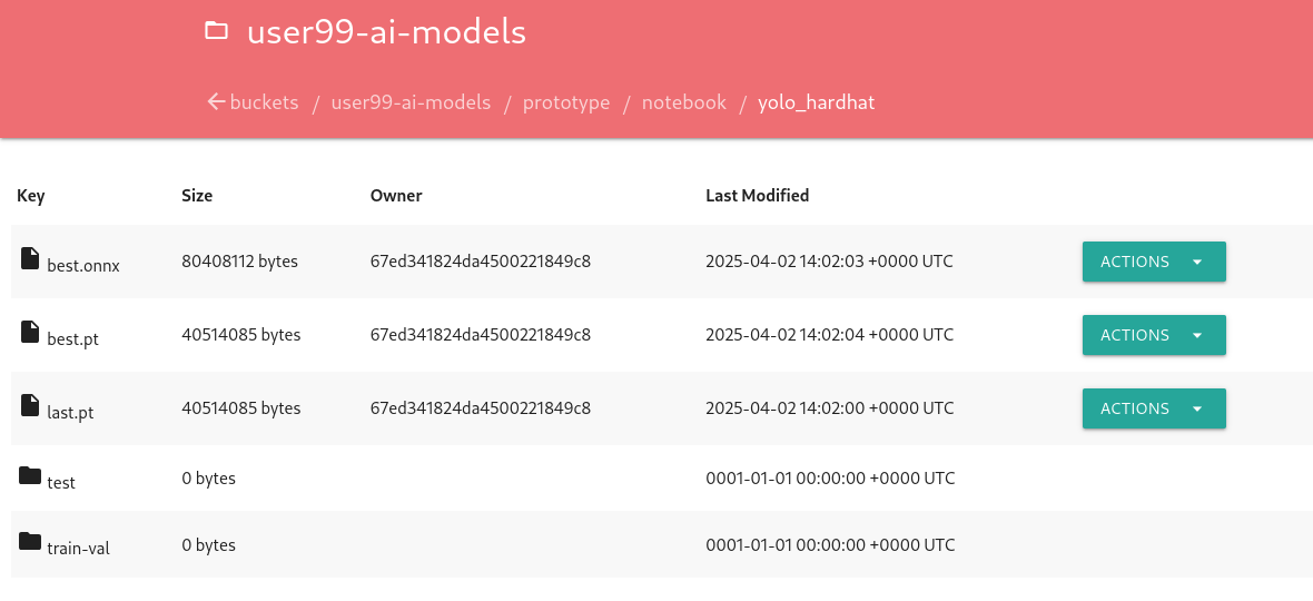
    upload_file(file_path, f"prototype/notebook/{directory_name}/test/{os.path.basename(file_path)}")

To facilitate easy verification of files uploaded to the object bucket, the workshop includes a (Web UI to browse the bucket contents.

You can go to that console ( https://s3-browser-USERNAME-ai-models-USERNAME-tools.apps.$CLUSTER_DOMAIN ) and open the prototype/notebook folder. You will find a folder with the "model train name" and inside you will have the model with the best performance metrics (best.pt) and the last produced with the last training epoch (last.pt) along with the performance stats for the Test, Validation and Training sets.

Finally, I recommend cleaning up the directories created during the training and evaluation processes to save some space. To achieve this, include a final piece of code in your Notebook that removes these directories.

!rm -rf {model_path_train}
!rm -rf {model_path_test}

Prototyping Pipeline (optional)

So far, you’ve used a Jupyter Notebook for quick model prototyping. While this approach is excellent for experimentation, transitioning to a more structured and scalable workflow can bring numerous benefits even for prototyping, such as ensuring consistency, repeatability, and improved collaboration.

OpenShift AI integrates seamlessly with Elyra Pipelines, an Open Source visual pipeline editor that simplifies the creation, editing, and execution of data science workflows. Elyra allows you to design workflows through an intuitive drag-and-drop interface, standardize your prototyping process to ensure reproducibility, and automate repetitive tasks to reduce manual effort. It also enables you to scale your workflows efficiently using OpenShift AI’s powerful infrastructure while making it easier to share and collaborate with your team.

Let’s build an Elyra Pipeline to automate the model prototyping process, helping you focus on innovation rather than managing infrastructure and repetitive tasks.

Custom Container Image

Using custom container base images in your pipeline tasks is a great idea because it eliminates the need to install dependencies every time the pipeline runs. This approach not only saves time but also reduces bandwidth usage, making your workflows more efficient and reliable.

By creating a custom container base image, you can preconfigure the environment with all the required dependencies for tasks like running Jupyter Notebooks. This means you won’t have to repeatedly set up the environment, ensuring a smoother and faster execution of your pipelines.

The first step is to create a Containerfile tailored for OpenShift. In this example, we’ll use a base image prepared for PyTorch and install the necessary dependencies such as Ultralytics, and Roboflow. The resulting Containerfile would look something like this:

FROM quay.io/modh/odh-pytorch-notebook:v2-2024a-20250116-b42b86c

USER 0

RUN INSTALL_PKGS="ultralytics roboflow" && \
    pip install --no-cache-dir  $INSTALL_PKGS

USER 1001

Then you can build your Container Image using the Containerfile and push it into a Container Image Registry (ie. Quay)

podman build -t <registry>/<namespace>/<image-name>:<image-tag> .
podman login -u <username> <registry>
podman push <registry>/<namespace>/<image-name>:<image-tag>

If you don’t want to build the image yourself, you can use an existing pre-built image: quay.io/luisarizmendi/pytorch-custom-notebook:latest.

Once you have the container image you want to use for running the code in your pipeline steps, the next step is to "import" it into your Jupyter environment for use with Elyra Pipelines.

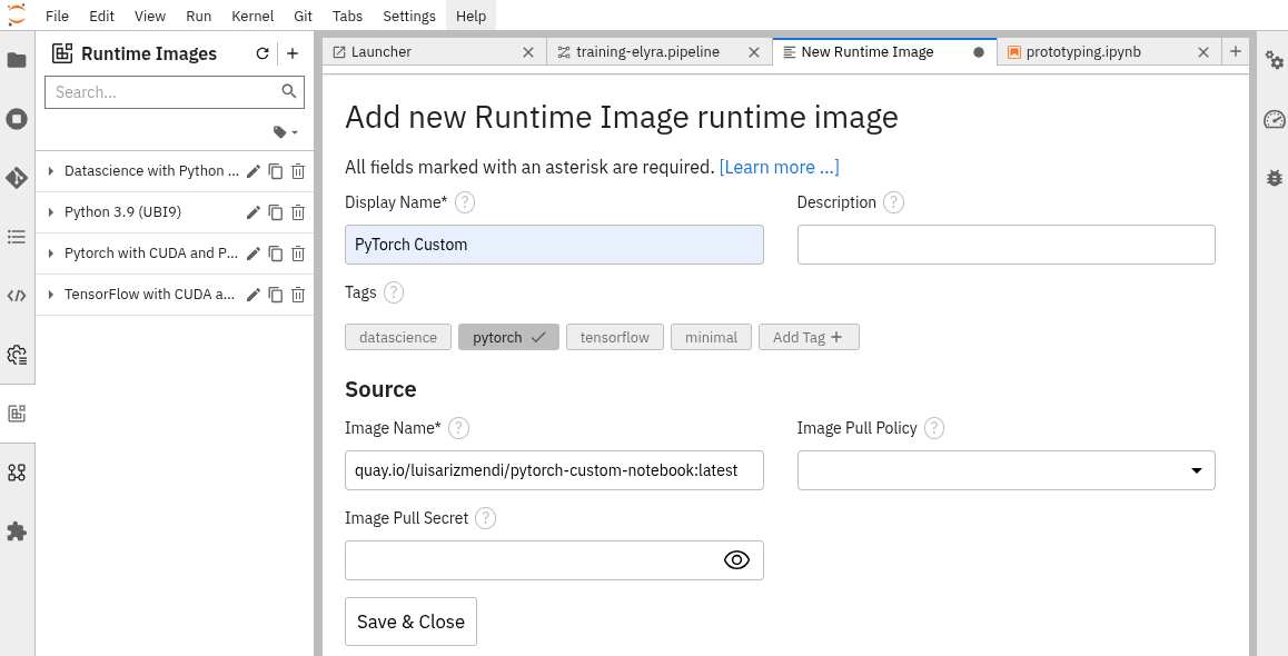
To add your custom image to the Jupyter Enviroment in order to use it with the Elyra Pipeline:

Open the Jupyter Notebook workbench.
Navigate to "Runtime Images" by selecting the icon with squares in the left menu.
Click the + button to add a new runtime image.
Provide a name for the image, such as PyTorch Custom, add a tag like pytorch, and specify the image name (e.g., quay.io/luisarizmendi/pytorch-custom-notebook:latest).
Click Save.

Once added, your custom container image will be available for use in your pipeline steps.

Pipeline Server

If you want to run Pipelines in OpenShift AI, you will need to add into your AI project a Pipeline Server resource definition.

To create a Pipeline Server:

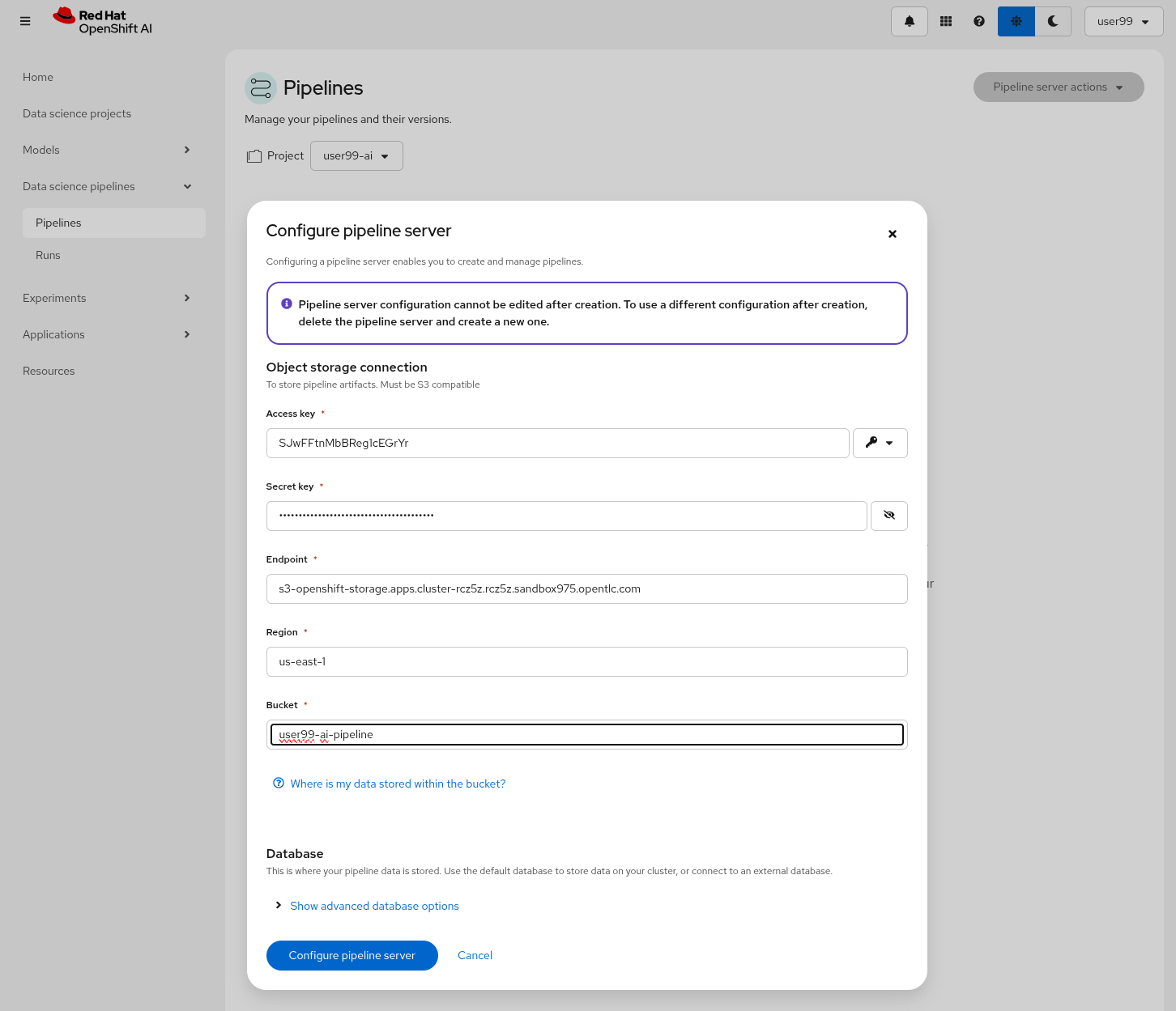
1- Navigate to "Data Science Pipelines > Pipelines" in OpenShift AI and configure a new pipeline server. Be sure that you are in the right project (USERNAME-ai).

Double-check that you are in the right Project: USERNAME-ai

2- Fill in the Data Connection information:

Access key: OBJECT_STORAGE_PIPELINE_ACCESS_KEY
Secret key: OBJECT_STORAGE_PIPELINE_SECRET_KEY
Endpoint: s3-openshift-storage.apps.CLUSTER_DOMAIN
Region: Keep the Region. If there is any pre-selected include any string (e.g. local).
Bucket: USERNAME-ai-pipeline

3- Click "Configure pipeline server".

4- Once the configuration is ready, restart any running workbenches to apply the updates.

To verify that the Pipeline Server has been successfully loaded into your Jupyter Environment, open the Workbench and navigate to "Runtimes" (represented by a gear icon in the left menu). Here, you can confirm that the runtime configuration has been automatically loaded. If the Data Science Pipelines runtime configuration is empty try to restart your workbench once the pipeline server is active.

Create the Pipeline Step Jupyter Notebooks

A pipeline is composed of multiple steps. In our case, it will consist of three: one step to fetch the dataset, another to train the model, and a final step to upload the files to the Object Storage. For this, you’ll need to create three new .ipynb files each corresponding to one of these steps.

To simplify the process, we’ll use the Jupyter Notebook created for quick prototyping as a base. However, this notebook cannot be directly split into pipeline steps. In a pipeline, each step runs independently, so you’ll need to incorporate mechanisms to transfer files and variables between steps.

This exercise will also help you prepare for implementing the training pipeline with Kubeflow, which will be covered in the Model Training section.

Start by copying the relevant code blocks from the prototyping notebook into their respective new files. Then, apply the necessary modifications as outlined below

If you prefer to save time, you can skip this step and directly reference the solution by using the pipeline files provided in the resources directory.

"Get Data" Notebook

Remove the pip install entries: Since you will be using the custom image that you created, you won’t need to install any further dependencies
Save the dataset variable into a file (eg, using pickle) since it will be used in the "Train" Notebook

import pickle

with open('dataset.pkl', 'wb') as file:
    pickle.dump(dataset, file)

"Train" Notebook

Include the relevant imports (this is a new Notebook, it does not use them from the "Get Data" Notebook)
Including environment variables is a great way to control the training configuration when launching the pipeline. For instance, you can define variables for parameters like the number of epochs and the batch size.

    'epochs': os.getenv("MODEL_EPOCHS"),
    'batch': os.getenv("MODEL_BATCH"),

As with the previous file, you need to save the variable containing the training and testing results so it can be used by the next step in the pipeline. However, due to the complexity of this variable, pickle cannot be used. Instead, you’ll need to manually serialize the data as shown below.

results_train_serializable = {
    "maps": results_train.maps,
    "names": results_train.names,
    "save_dir": results_train.save_dir,
    "results_dict": results_train.results_dict,
}

results_train_save_path = "model_train_results.pth"

torch.save(results_train_serializable, results_train_save_path)

results_test_serializable = {
    "maps": results_test.maps,
    "names": results_test.names,
    "save_dir": results_test.save_dir,
    "results_dict": results_test.results_dict,
}

results_test_save_path = "model_test_results.pth"

torch.save(results_test_serializable, results_test_save_path)

"Save Data" Notebook

Again, include the relevant Python imports.
Deserialize the variables that were stored in a file in the "Train" Notebook:

import torch

results_train_save_path = "model_train_results.pth"
results_train = torch.load(results_train_save_path)

results_test_save_path = "model_test_results.pth"
results_test = torch.load(results_test_save_path)

The deserialized values are accessed as an array rather than through methods. Therefore, you’ll need to update results_xxx.save_dir to results_xxx['save_dir']`:
Update the path where the model and results are stored in the Object Storage (e.g., change from prototype/notebook/ to prototype/pipeline/).
Since the pipeline will run multiple times using the same storage, it’s recommended to clean up the generated files after the pipeline has finished saving the content.

Create an Elyra Pipeline

It’s time to create the Pipeline with the files that you prepared.

To create a new Elyra pipeline do the following in your Workbench:

1- Right-click on the directory view where the pipeline step files are located and select "New Data Science Pipeline Editor". Alternatively, you can open a new tab by pressing + and selecting "Pipeline Editor" from the Elyra section.

2- Rename .pipeline file to training-elyra.pipeline.

3- Drag-and-drop the Step files that you prepared and connect them in the right order.

4- Click the square with an arrow inside at the top right corner. A new menu will appear on the right with several tabs for configuring the pipeline and its steps. When you click a step, its configuration will open. You need to configure the following:

At the general pipeline level configure a "Data Volume" so the steps can share the files (it should be mounted under /opt/app-root/src) and the general Runtime Image that will be used, in this case it will be the custom image that you created (PyTorch Custom).

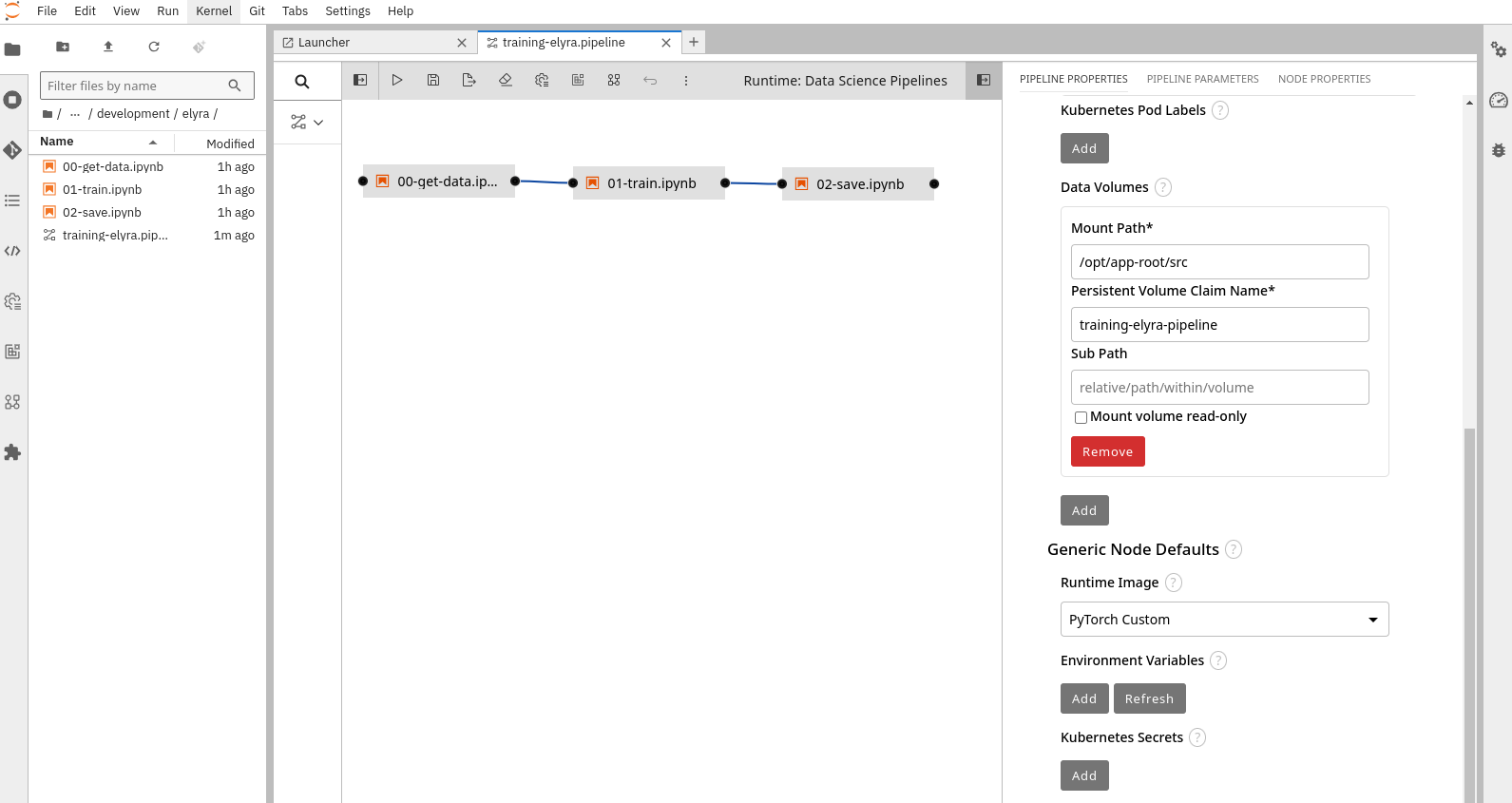
The training-elyra-pipeline Persistent Volume is not autogenerated, so you will need to manually create the Persistent Volume Claim with the specified name in the project where the pipeline will run ("USERNAME-ai"), otherwise the pipeline won’t progress when you launch it.

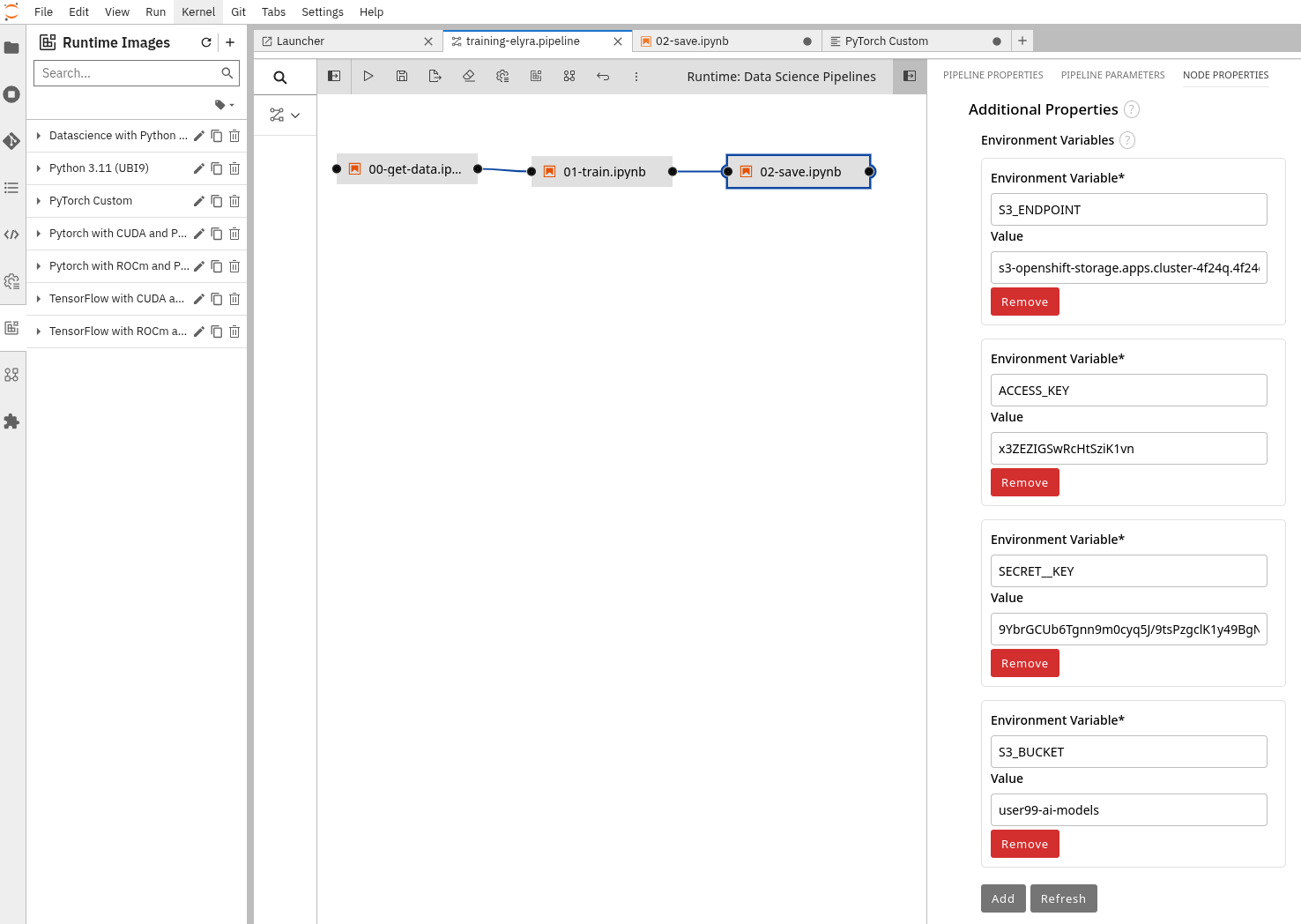
In each step you will need to fill in the required Environment Variable values that will be used, in our example:
- In the "Get Data" step: ROBOFLOW_KEY, ROBOFLOW_WORKSPACE, ROBOFLOW_PROJECT and ROBOFLOW_DATASET_VERSION
- In the "Training" step: MODEL_EPOCHS and MODEL_BATCH
- In the "Save Data" step: AWS_S3_ENDPOINT, AWS_ACCESS_KEY_ID, AWS_SECRET_ACCESS_KEY and AWS_S3_BUCKET

Remember that if you want to save time you could use the "Mock Training" Dataset (although it produces a non-usable model).

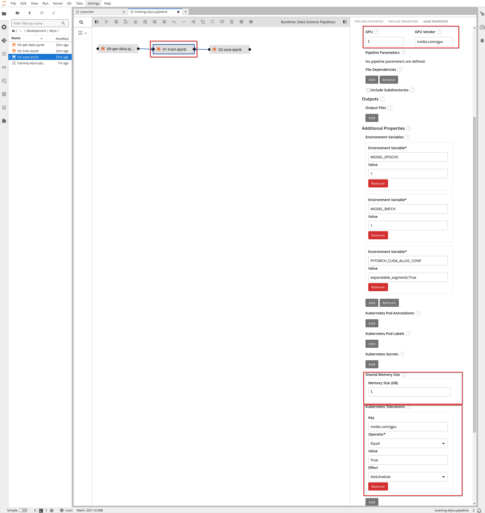
5- If you are running in an environment with GPUs, you must:

Specify the GPU number and GPU Vendor (nvidia.com/gpu) in the training task.
If there are Kubernetes Taints in the GPU nodes you will also need to configure the Toleration. GPUs will be used during training, but you should include the Toleration in all tasks. This is necessary for Kubernetes to schedule the pod on a GPU-enabled node. Since tasks share a Persistent Volume (PV), there is a risk that GPU nodes may be in a different zone where the PV cannot be shared with non-GPU nodes. If this happens, Kubernetes will always select a node without GPUs, or you may encounter an error if scheduling is forced.
Add additional Shared Memory Size in the Training Task.

6- Click save (icon with a disk on the top menu).

If you want to play a little bit more with the Elyra Pipelines, try to modify the code to get more inputs (environment variables) to, for example, let configure dynamically the optimizer or the learning rate.

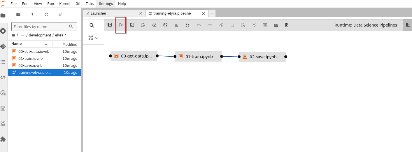
Run the Elyra Pipeline

It’s time to run you Pipeline (click the "play" button on the top bar menu).

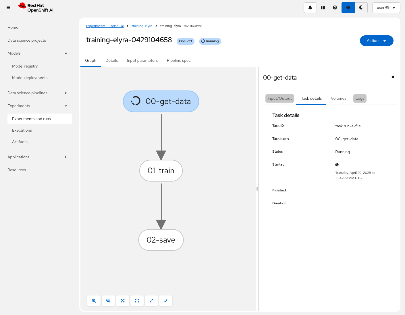
After running the pipeline, you can see the progress in the OpenShift AI console.

You can see the Pipeline progress by:

Navegating to OpenShift AI: https://rhods-dashboard-redhat-ods-applications.apps.CLUSTER_DOMAIN
Selecting the Pipeline name in "Experiments and runs".
Opening the running task.

The first time that you run the Pipeline it could take some time to finish the first task since it needs to pull the custom Container Image.

You can only view the logs of the tasks once they are completed. However, if you’re interested in monitoring the logs in real time, you can access the Pod logs directly through the OpenShift Console.

You can use the logs of the training task to check if the GPU is being used:

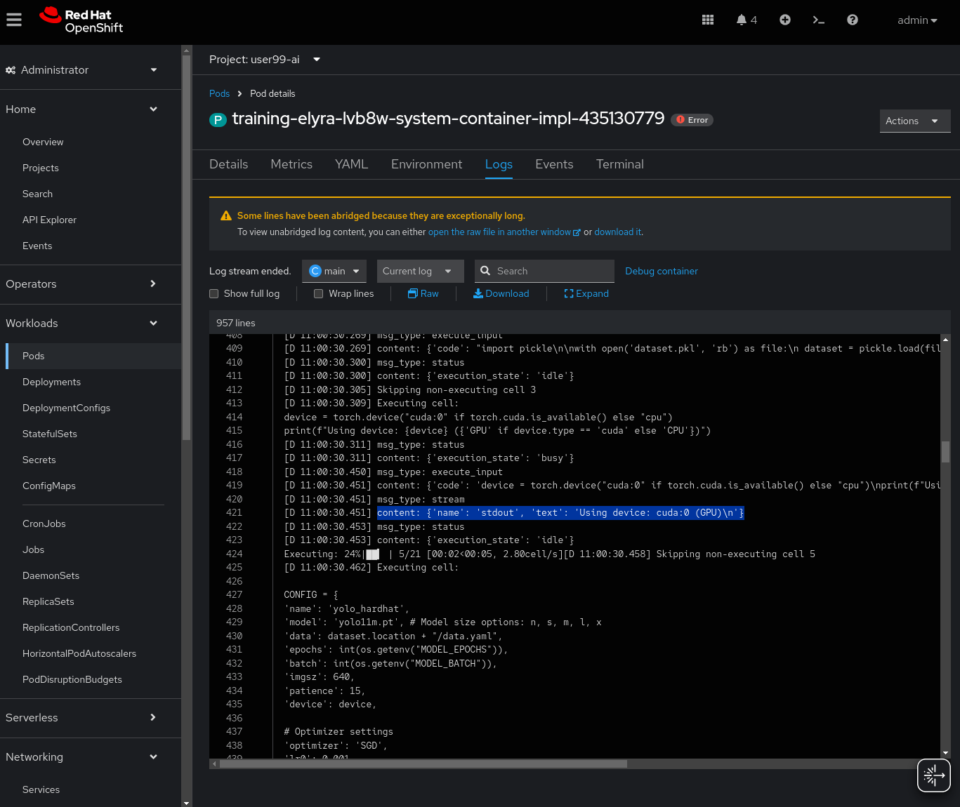
Once the Pipeline is finished, you could check that the contents are saved into the Object Data Store by navigating to ( https://s3-browser-USERNAME-ai-models-USERNAME-tools.apps.$CLUSTER_DOMAIN ) and open the prototype/pipeline folder.

Solution and Next Steps

In this section, you created an initial prototype of the model by training it with different hyperparameter values to explore its potential. If the performance metrics obtained are not satisfactory, or if you used the "Mock Training" dataset with a reduced set of images, you can now download and utilize the version 1 of the pretrained model.

You can now also push to the Git Source repository the files that you created:

Click on the Git icon on the left menu.
Press the + to select the files to be pushed.
Include at the botton the Commit message.
Press "Commit".
Use the Git menu in the top bar to Push the changes into the remote repository.

Finally, since you won’t need it in further steps, it’s a good idea that you stop the OpenShift AI Workbench that you have been using to save resources in the OpenShift cluster.

Move on into Model Training.